Human log loss for image classification

Deep learning vs human perception: creating a log loss benchmark for industrial & medical image classification problems (e.g. cancer screening).

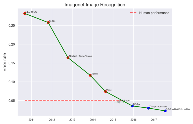
In the last few years convolutional neural networks have outperformed humans in most visual classification tasks. But there is one caveat – usually they win by a small margin:

There are few exceptions to this rule, including the whale individuals detection contest our deepsense.ai team won (85% accuracy for almost 500 different whales). However, one could argue that a computer’s pattern recognition skills were similar to a human’s, but it was easier for the computer to memorize 500 different whale specimens.
When we train our deep learning model for an image classification task, how do we know if it is performing well? One way to approach this problem is to compare it against a human performance benchmark. We expect human errors even for simple tasks – labels can be misclassified and the person performing the classification is likely to make mistakes from time to time: after all, “to err is human”.
Creating benchmarks for medical and industrial problems is even more challenging, because:

• we don’t have a simple sanity check (unlike distinguishing dogs from cats),
• it is not obvious if a single photo devoid of any context is enough for classification (very often even for the best specialists it is not).

Measuring human accuracy for medical images

In the Cervical Cancer Screening Kaggle competition (by Intel & MobileODT), the goal was to predict one of three classes of cervical openings for each patient. To see this image classification task, visit (warning: explicit medical images) Cervix type classification or this Short tutorial on how to (humanly) recognize cervix types.
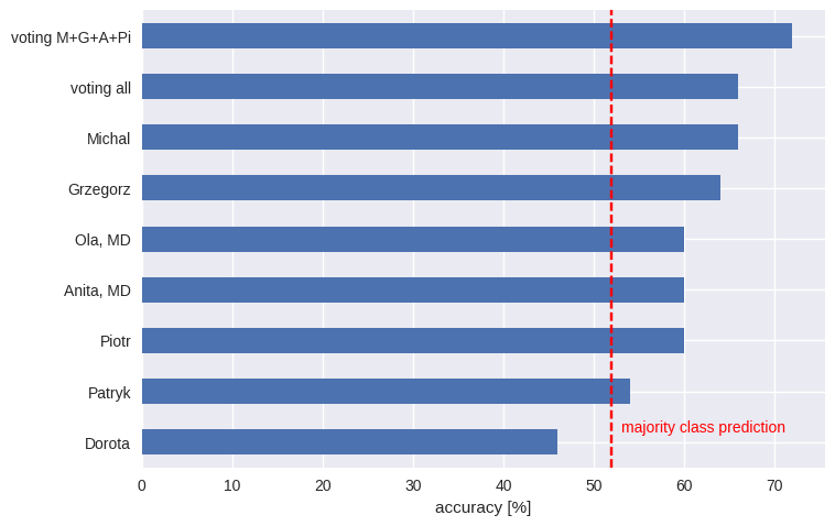
Our networks in this competition were just a bit better than a random model. We wanted to quantify human performance to see if our networks were bad, or if it is simply impossible to do much better. To measure human accuracy, we sampled 50 cervix images. This number sounded like a reasonable trade-off: high enough for some estimations, but small enough not to exhaust us. Unlike Andrej Karpathy, who set the human benchmark for ImageNet, we avoided going through the whole dataset. We looked at them ourselves and also gave them to two medical doctors, one a gynecologist.  The task was to predict the cervix opening class for each image. The accuracy was as follows:

At least most of us did better than using the majority class prediction – i.e. assigning each image to the most numerous class. The medical doctors didn’t outperform the rest of us. That may seem surprising, but there is a common phenomenon at work here: many visual task  much knowledge, just good pattern recognition (even pigeons can detect cancer from photos). Even less unexpected is the wisdom of crowds – an ensemble model (which involves members of “the crowd” voting) significantly outperformed each individual prediction.

Translating categorical predictions into log loss

However, many machine learning tasks use another measure of error – log loss (also known as cross-entropy), which takes into account our uncertainty (e.g. it is better to predict the correct class with 90% certainty than with 51%). It is especially important for problems with imbalanced classes. If we want to use the same prediction for a group of items, to minimize log loss we need to use empirical probabilities for the sample.  For the whole sample of cervixes, those probabilities would be (18%, 52%, 30%) for classes 1, 2 and 3, respectively, resulting in a log loss of 1.01.
To measure human log loss we need to ask people to predict a probability distribution for each image, e.g. (20%, 70%, 10%). However, this task is time-consuming and can be difficult to explain to non-data scientists, in this case medical doctors. Humans are notoriously bad at assigning probabilities, so this approach would most likely need calibration anyway.
Fortunately, there is a very simple probability calibration technique, which takes discrete predictions as its input. Here’s the recipe:

• predict a class for each image (here: 1, 2 or 3)
• for all instances with the same predicted class, calculate the empirical distribution of the ground truth values
• turn discrete predictions into the respective distributions
• given the predictions, calculate the log loss

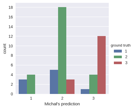
For example, for Michał (the project leader and top guesser), it is:

So, whenever he predicted class 1, we assign it to the (3/7, 4/7, 0/7) probability distribution, for class 2 – (5/26, 18/26, 3/26) and for class 3 – (1/17, 4/17, 12/17). His log loss on the same dataset is 0.78. This procedure is equivalent to calculating the conditional entropy of cervix classes, given our prediction, that is: H(groud_truth | our_prediction). See also the Wikipedia page on mutual information and its relation to conditional entropy.

Human predictions vs Kaggle results

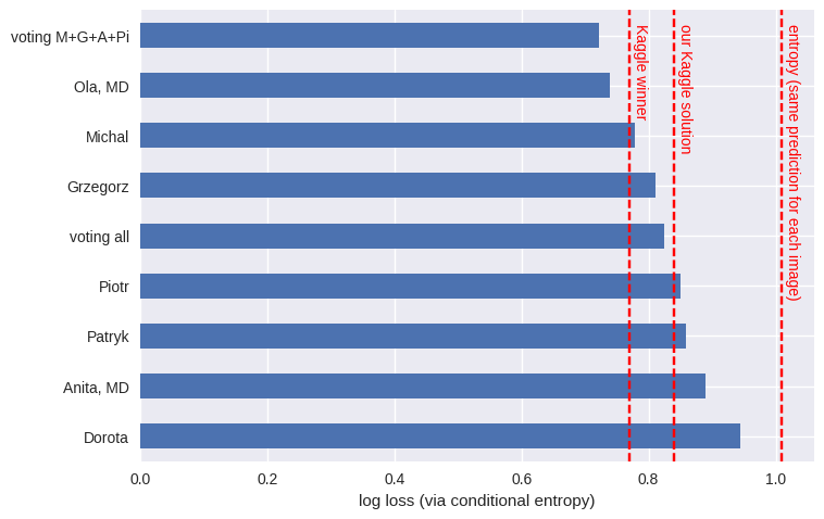
Here we calculate the conditional entropy for each participant:

How does this compare to the final Kaggle results? Ultimately, the top winner had a log loss of 0.77, whereas our (artificial, not biological) neural network ensemble returned 0.84. Neither of those beat us humans, with our log loss of 0.73.
During the competition phase had seen entries with log loss as low as 0.4. We hadn’t known if the authors had used a clever approach, or if it had been simply an overfit. After our human test, however, we rightfully assumed that it was indeed a large overfit. It seems that this technique may be useful for setting a reasonable benchmark for your next image classification problem – whether it’s a Kaggle challenge or a project for your customer.

Additional materials

Remarks

• This technique may underestimate log loss (in general, there is no unbiased estimator for Shannon entropy). A more educated way (but one requiring more samples) would be to use cross-validation. To avoid ending up with zero probabilities, smoothing probabilities may be crucial.
• We can use different classes for guessing than when we want to predict, for example, using the option “I don’t know”. The magic of methods related to entropy is that they are label-insensitive.
• To learn more about entropy, read the first two chapters of Thomas M. Cover, Joy A. Thomas, Elements of Information Theory.

Code snippet

import numpy as np
from sklearn.metrics import confusion_matrix
# label - ground truth labels
# predictions - prediction labels
def entropy(x, epsilon=1e-6):
    # assumes x is normalized
    return (- x * np.log(x + epsilon)).sum()
def conditional_entropy(mat):
    mat = mat / mat.sum()
    return entropy(mat) - entropy(mat.sum(axis=0))
print(conditional_entropy(confusion_matrix(label, prediction)))

Project members: Michał Tadeusiak (leader), Grzegorz Łoś, Patryk Miziuła, Dorota Kowalska, Piotr Migdał.
Thanks also to Robert Bogucki, Paweł Subko and Agata Chęcińska for valuable remarks on the draft.